How to display graphics#

On one hand, you write exercises as pure batch-oriented applications. This means that no interactive display nor graphical output are expected when your exercises are executed, only a textual signature is expected.

On the other hand, in order to visually check algorithms and results, you are asked to add graphical output in a common application named display.py, keeping the exercises themselves without graphics.

The favourite approach to manage the two aspects of the development will be therefore to factorize the base features of each exercise into a shared library, which will be used both in the exercice solution and in the display.py application.

In this section we give you a set of hints about

how to structure your graphical application
how to develop some usual graphical properties by which you’ll present test values
how interact dynamically with your display application and its data

Architecture of the graphical application#

A graphical application is composed of

some import statements meant to connect to the matplotlib libraries
a descriptive section to setup the graphical components where data will be presented
some callback functions which will be triggered whenever some interactive actions are activated (clicks, moves, etc…)
a global and unique show action that commits all graphical orders.

import matplotlib.pyplot as plt

def minimal() -> None:
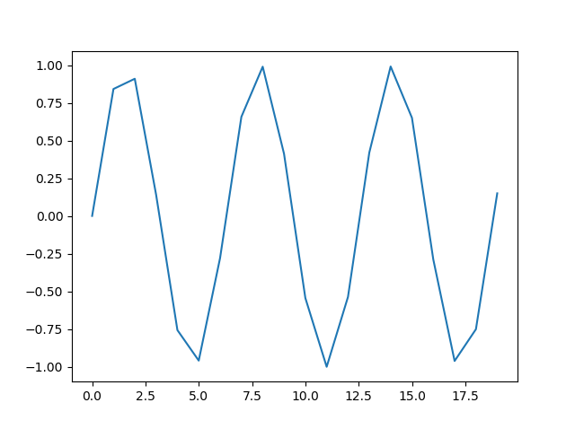
  """ Simply plot a sinusoid into one single drawing area """
  plt.plot(np.sin(np.arange(0, 20.0)), label="sin values")
  plt.legend()
  plt.show()


if __name__ == '__main__':
  minimal()

The main component : the “axe”#

In the context of the matplotlib library, one central component holds the graphical actions. It’s called the axe since its describes an oriented coordinates system.

Thus, you first create some axe objects, you position them onto the screen, you draw into them, and you may interact with them individually.

To position the axe, you design a rectangular matrix (ie. as rows & columns) and every axe will occupy one or more cells in this matrix. Cells are indexed as (column, row) where the (0, 0) cell is at the top left position.

Be carefull that the local coordinate system of one individual axe is different than the convention used to index the cells: The zero of the y local coordinate is at the bottom of the cell !!!

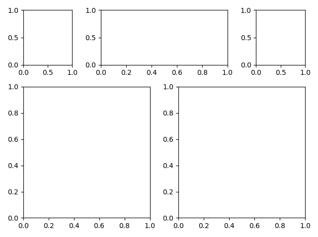
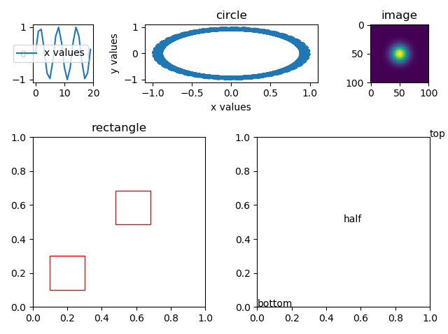
In the following example, we design 3 x 4 cell matrix, and we position 5 axes onto it. Some axes span some adjacent rows or columns.

import matplotlib.pyplot as plt

def draw(axe_1, axe_2, axe_3, axe_4, axe_5) -> None:
    """Draw someting."""
    # Here will come various drawing operations...
    pass

def display() -> None:
    """Display figure with empty subplots.

    (for test purposing)
    """
    axe_1 = plt.subplot2grid((3, 4), (0, 0))
    axe_2 = plt.subplot2grid((3, 4), (0, 1), colspan=2)
    axe_3 = plt.subplot2grid((3, 4), (1, 0), colspan=2, rowspan=2)
    axe_4 = plt.subplot2grid((3, 4), (0, 3))
    axe_5 = plt.subplot2grid((3, 4), (1, 2), colspan=2, rowspan=2)

    draw(axe_1, axe_2, axe_3, axe_4, axe_5)

    plt.tight_layout() # To nicely occupy the screen
    plt.show()         # Nothing is actually displayed before this call.


if __name__ == '__main__':
    display()

Some usual graphical facilities#

Onto a given axe, one may

plot: draw N-dimension data
text: draw text
add_patch: draw geometrical figures
legend

The matplotlib documentation is huge, but offers many ways to discover all possible graphical features or data presentation utilities. We encourage you to widely explore the very nice example galery, and the set of tutorials (tutorials https://matplotlib.org/gallery/index.html).

Here we simply present the basics of the display.py application that you will be continuously extending throughout the course.

import matplotlib.pyplot as plt
import matplotlib.patches as patches

def draw(axe_1, axe_2, axe_3, axe_4, axe_5) -> None:
    """Plot basic subplots example."""
    # 1-D plot
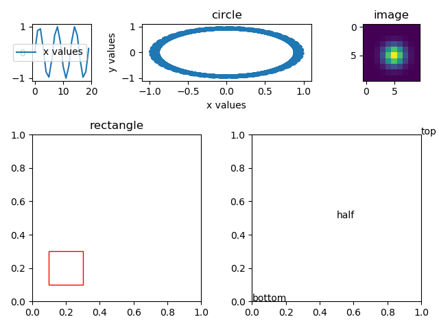
    axe_1.plot(np.sin(np.arange(0, 20.0)), label="x values")
    axe_1.legend()

    # 2-D plot
    axe_2.plot(np.sin(np.arange(0, 200.0)), np.cos(np.arange(0, 200.0)))
    axe_2.set(title="circle", xlabel="x values", ylabel="y values")

    # Display an image (ie. a 2D matrix of pixels)
    image = create_image()
    axe_4.set(title="image")
    axe_4.imshow(image)

    # create a graphical object (a rectangle) and add it to one of the drawing zone
    center = (0.1, 0.1)
    rect = patches.Rectangle(
          center,
          width=2 * 0.1,
          height=2 * 0.1,
          fill=False,
          color="red"
    )

    axe_3.set(title="rectangle")
    axe_3.add_patch(rect)

    # Add some texts
    axe_5.text(x=0., y=0., s="bottom")
    axe_5.text(x=0.5, y=0.5, s="half")
    axe_5.text(x=1., y=1., s="top")

def f() -> None:
    ...
    # Various examples of graphical actions that can be drawn into zones
    axe_1.imshow(pixels)       # 2D array
    axe_2.plot(x, y)           # contour
    axe_3.fill(x, y)           # Filled contour
    axe_4.hist(x, numb_bins)

    axe_5.fill(x, y1)          #
    axe_5.plot(x, y2)          # Sharing an axe superimpose drawings
    axe_5.hist(z, bins)        #

    axe.set_xlabel("...")
    axe.set_ylabel("...")
    axe.set_title("...")

    plt.plot(x, y)              # Act upon the most recent axe

Interactivity in the graphical display#

To interact with graphics, we declare callbacks (ie. functions only called by the system whenever some interactive actions are detected (such as clicks, mouse moves, etc.)

All callback f unctions follow the same form, ie. they receive one event object argument that contains the context upon which the event was detected:

the axe onto which the action was issued (field = inaxes)
the local (to the axe) coordinates of the event (field = xdata, ydata) . It should be noted that the coordinates of the event (ie. x, y of the cursor) are automatically converted to local coordinates.
plus some event specific details

Callback functions has to be declared once the axes are initialized, and before the graphics is realized.

def onclick(event) -> None:
   if (event.inaxes is not None) and (event.inaxes == axe_1):
        print("Click occured in axe_1 at x={} y={}".format(event.xdata, event.ydata))

...

fig = axe_1.figure
fig.canvas.mpl_connect('button_press_event', onclick)

Of course, due to the global aspect of the callbacks, we have to carefully manage the python variables, especially considering the axes variables. The simplistic approach consists in making those variables global, however this approach is not completely safe and should be avoided.

A much better approach would be to use a class based architecture… as follows:

class Display(object):
    def __init__(self):
        # Setup a drawing area, and declare a callback to receive the mouse motion events
        self.axe = plt.subplot2grid((3, 4), (0, 0))

        fig = self.axe.figure

        def onmove(event) -> None:
            print("moving...", event.xdata, event.ydata)
            pass

        fig.canvas.mpl_connect('motion_notify_event', onmove)

    def draw(self) -> None:
        plt.tight_layout()
        plt.show()

if __name__ == '__main__':
    d = Display()
    d.draw()

Several pre-defined graphical widget components. Widget components as some predefined graphical constructs, with properties, and behaviours (associated with callbacks)

from matplotlib.widgets import Button
from matplotlib.widgets import RadioButtons
from matplotlib.widgets import CheckButtons
from matplotlib.widgets import Slider
from matplotlib.widgets import Cursor

def widgets() -> None:
    """
    Button
    RadioButtons
    CheckButtons
    Slider
    Cursor
    Menu
    """
    def callback(event):
        print("Hello")

    # A widget has to be created in the context of an existing axe.
    b = Button(axes, "Hello")
    b.on_clicked(callback)

Zooming an image#

Images position and extension can be controlled using the limits. You must pay attention on how the coordinate system is applied to an image displayed onto an axe: the zero of the y coordinate is at top of the axe. Therefore, when querying the limits, you get the maximum value of the y coordinate first, and then the minimum value.

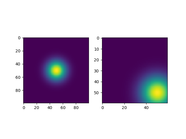
In the following example, we show two identical images. Then when we click on the left image, we zoom out the right image. In addition, we show the zoomed region as a red rectangle on the left image.

class Zoom():
    def __init__(self):
        """
        We define two drwaing areas, onto which the same image is drawn.
        then, a callback receives the click selectively fro the left area
        Upon this click, the right area is zoomed in.
        """
        self.fig = plt.figure()

        self.axe_1 = plt.subplot2grid((1, 2), (0, 0))
        self.axe_2 = plt.subplot2grid((1, 2), (0, 1))

        image1 = create_image()
        image2 = create_image()
        self.axe_1.imshow(image1)
        self.axe_2.imshow(image2)

        self.xmin1, self.xmax1 = self.axe_1.get_xlim()
        self.ymax1, self.ymin1 = self.axe_1.get_ylim()
        self.xmin2, self.xmax2 = self.axe_2.get_xlim()
        self.ymax2, self.ymin2 = self.axe_2.get_ylim()

    def onzoom(self, event) -> None:
        # all click trigger this callback
        if (event.inaxes is not None) and (event.inaxes == self.axe_1):
            # if the click comes from the left area
            dwidth = 40.0
            dheight = 20.0
            # we redefined the limits for the right area to be smaller than the default ones
            self.axe_2.set(xlim=(self.xmin1, self.xmax1 - dwidth),
                           ylim=(self.ymax1 - dheight, self.ymin1),
                           autoscale_on=False)
            # print the evolution
            xmin2new, xmax2new = self.axe_2.get_xlim()
            ymax2new, ymin2new = self.axe_2.get_ylim()
            print(
              "zoom xmin1=", self.xmin1,
              " xmax1=", self.xmax1,
              " ymin1=", self.ymin1,
              " ymax1=", self.ymax1,
              " xmin2=", self.xmin2,
              " xmax2=", self.xmax2,
              " ymin2=", self.ymin2,
              " ymax2=", self.ymax2,
              " xmin2new=", xmin2new,
              " xmax2new=", xmax2new,
              " ymin2new=", ymin2new,
              " ymax2new=", ymax2new
            )

            # show the new limits as a red rectangle on the left area
            corner = (self.xmin1, self.ymin1)
            rect = patches.Rectangle(corner,
                             width=xmax2new - xmin2new,
                             height=ymax2new - ymin2new,
                             fill=False,
                             color="red")
            self.axe_1.add_patch(rect)
            self.fig.canvas.draw()

    def run(self):
        self.fig.canvas.mpl_connect('button_press_event', self.onzoom)
        plt.show()

Managing dynamics in the graphics#

In this chapter we discuss how to make the graphics configuration dynamics, in association with some interactivity.

Let’s consider the following situation:

the mouse passes over one of the axes
only on a selected axe, we draw a red rectangle around the cursor position
we want to follow the cursor motion
when the cursor passes right over some specific position of the selected axe (eg. the center), then we show the rectangle as green instead of red

You should notice that each time onmove is called, it must erase the rectangle previously drawn, before drawing any new one. Thus, we must remember the rectangle from one call to another (see the end of Python Classes Notebook) : this is why the variable rect is declared at the level of the class.

class Motion(object):
    def __init__(self):
        self.fig = plt.figure()
        lines = plt.plot(np.sin(np.arange(0, 20.0)), label="x values")
        line = lines[0]
        self.axe = line._axes
        self.rect = None
        self.xmin, self.xmax = self.axe.get_xlim()
        self.ymax, self.ymin = self.axe.get_ylim()

    def onmove(self, event) -> None:
        print("Motion occured in axe at x={} y={} {} {}".format(
          event.xdata,
          event.ydata,
          event.inaxes,
          self.axe)
        )
        if (event.inaxes is not None) and (event.inaxes == self.axe):
            print("Motion occured in axe at x={} y={}".format(event.xdata, event.ydata))

            if not self.rect is None:
                self.rect.remove()
                self.rect = None

            x = event.xdata
            y = event.ydata

            middle = (
                (self.xmax - self.xmin) / 2,
                (self.ymax - self.ymin) / 2,
            )

            color = "red"
            if (abs(x - middle[0]) < 1) and (abs(y - middle[1]) < 1):
                color = "green"

            half_width = (self.xmax - self.xmin) / 10.
            half_height = (self.ymax - self.ymin) / 10.
            corner = (x - half_width, y - half_height)
            self.rect = patches.Rectangle(corner,
                                  width=2 * half_width,
                                  height=2 * half_height,
                                  fill=False,
                                  color=color)

            # axe_3.set(title="rectangle")
            self.axe.add_patch(self.rect)
            self.fig.canvas.draw()

    def run(self) -> None:
        self.fig.canvas.mpl_connect('motion_notify_event', self.onmove)
        plt.show()

class OnMove(object):

    def __init__(self, a):
        self.rect = None

    def __call__(self, event):
        if not event.inaxes is None and event.inaxes == axe_3:

            print("Motion occured in axe_3 at x={} y={}".format(event.xdata, event.ydata))

            if not self.rect is None:
                self.rect.remove()
                self.rect = None

            x = event.xdata
            y = event.ydata

            color = "red"
            if (abs(x - 0.5) < 0.05) and (abs(y - 0.5) < 0.05):
                color = "green"

            half_size = 0.1
            corner = (x - half_size, y - half_size)
            self.rect = patches.Rectangle(corner,
                         width=2 * half_size,
                         height=2 * half_size,
                         fill=False,
                         color=color)

            # axe_3.set(title="rectangle")
            axe_3.add_patch(self.rect)
            rect.figure.canvas.draw()

    ...

    fig.canvas.mpl_connect('motion_notify_event', OnMove())

NPAC Computing Course

How to display graphics

Contents