Find the peaks
Contents
Find the peaks#
Reminder
Start the exercise with the Python template file in the
srcdirectory corresponding to the exercise.
Your code must be added to the
mainfunction.If you write generic functions, put them into libraries to reuse them easily in other applications. Look at Library and Module documentation for more details on Python libraries.
You should carefully follow the division in steps proposed for every exercise and provide specific signatures for each step when this is specified.
Git operations:
Commit very frequently with relevant message. Focus on making clear the reasons why you made the change.
Push once a significant result is obtained.
Code quality:
Check frequently the PyCharm annotations about your code, for example the colored signals in the right vertical gutter.
Execute the
check_commit_status.pyscript to check the validation tests.Assess the quality of your code with SonarQube.
Documentation:
Add docstrings (
""" ... """) at begining of ALL functions & classes.Add one-line comments wherever this is useful to understand your code.
Refer to slides for detailed information on technical topics.
Goal#
Before trying to recognize the celestial objects present on a image (later exercises), one must first analyse the image, in search for peaks, i.e. pixels whose value is greater than their neightbors. So to find them more precisely, one can reduce the image noise by convoluting it with a fixed gaussian pattern.
Principle#
An image is a 2D array of pixels. We want to identify all regions of this image, made of contiguous pixels, called clusters. (These regions will be later on associated with celestial objects we want to characterize).
Remark: Of course, the definition of a cluster presented here is very simplistic. In real searches, much more sophisticated algorihms are used. However, this is sufficient to give a realistic vision of the process used in astronomy.
To identify the contiguous pixels, only the pixels with a luminosity value greater than a threshold are considered.
To isolate and identify all these regions, we decompose the algorithm in several steps:
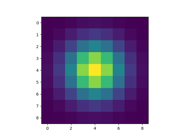
We construct a 2D normalized sharp gaussian pattern (i.e. whose integral is 1.0)
We first extend the image by adding a margin of extra pixels all around it, so as to limit the side effects at the borders of the convolution algorithms. In principle, those extra pixels should preferably be filled in using background values. However for practical reasons, we simplify this and just fill it with zeroes. This impact is negligible in our case, but should considered when working on a real physics case.
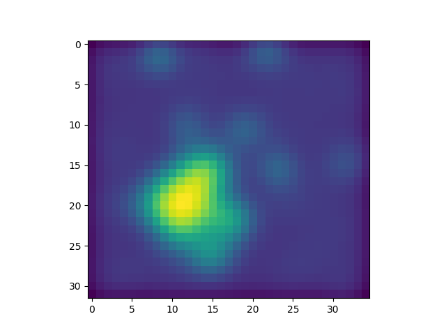
We then build a convoluted image derived from the raw image, and having the same shape (size):
This is obtained by doing a 2D linear scan of the image grid, (line by line: the first row is scanned, then the second one…)
At each position, a scalar value is computed by doing a convolution operation as follows:
a 9x9 sub-image is extracted from the raw image, centered at the scan current position (thus possibly including the added margin pixels when the scan position is close to the image border).
Then, the convolution consists in multiplying the gaussian pattern by this sub-image (using element by element multiplication) and summing the resulting pixels.
all those scalar values are stored in the convoluted image.
The convoluted image is scanned to detect peaks as follows:
A peak exists when and only when the intensity value of a pixel is strictly greater than all the immediately surrounding pixels.
Note that here again, we have to slightly extend (by one pixel, due to the previous definition) the convoluted image so as to limit the side effects close to the image borders.
We should also ignore peaks below the threshold.
Around each peak position, in the original raw image, all the contiguous pixels above the threshold are collected into a cluster.
This exercise limits itself to the identification of peaks. The next exercise will no longer need the convoluted image, and we will go back to work with the real pixels, and will construct clusters around peaks positions.
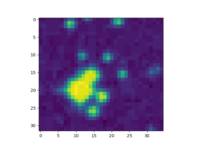
In the explanations below, we will consider one image to exemplify the steps of the exercise:
Implementation details#
As for every exercise, you will import the modules developed for the previous exercises.
You should also put the functions for this exercise in a dedicated module named lib_peak.py.
And the main program should be written in a file ex3_peaks.py.
About coordinate systems#
During this exercise and the following ones we will use several coordinate systems, depending on the context:
Image coordinates: they are expressed as a
(x,y)tuple representing the position of the pixel based on a reference position(x=0,y=0)at the upper-left corner of the displayed image (as displayed for example by amatplotlib.pyplot.imshow()function), the x axis being horizontal and the y axis being vertical.NumPy coordinates: they are used to locate an element in a 2D array. This is a set of 2 indexes:
[r][c]:r(row) matching theycoordinate of the image coordinate systemc(column) matching thexcoordinate of the image coordinate system.
This must be taken into account when a
NumPycoordinate has to be used in the other contexts: The origin ([r=0][c=0]) matches the image origin ((x=0,y=0)).Display coordinates: they are expressed as a
(x,y)tuple like image coordinates. But here, the reference ((0,0)) is the lower-left corner of thePyPlotwindow and the unit is different (display pixel instead of image pixel with a ratio between them depending on the “zoom” factor of the image).
When using coordinates, pay attention to use the appropriate coordinate system.
Additional slides and notebooks#
Some slides are needed to complete this exercise and to get more precise technical information. Sometimes it may even be also needed to explore the complete documentations that are shown in appendices. Here: Fits slides, Numpy Notebook, Pyplot slides are very useful.
Step 1: build the gaussian pattern#
Create a build_pattern() function to build a 2D matrix (pattern). This
is a 2D (9x9) matrix with a normalized gaussian pattern. This odd size is
selected so as to ensure that the pattern offer a single pixel at its center.
To create the pattern matrix, you will have to use Numpy. The proposed method is:
Create two 1D vectors of size 9 using the
numpy.arange()function. The first one describe the 9 values for theXaxis, while the second one describes the 9 values for theYaxis. But, to make it a real vertical axis, you have to transpose it using the expressiony = y[:, numpy.newaxis](Seenumpy.newaxis).Take advantage of the one-dimensional Gaussian function defined in the lib_model module to build the two-dimensional Gaussian function:
\[\mathcal{G}_{2D}(x,y) = \mathcal{G}_{x}(x)\mathcal{G}_{y}(y) = A_x A_y \exp\left( -\left(\frac{(x - x_0)^2}{2\sigma_x^2} + \frac{(y - y_0)^2}{2\sigma_y^2} \right)\right)\]Pass the
XandYorthogonal vectors as arguments of the gaussian functions to create a 2D matrix containing all \(\mathcal{G}_{2D}(x,y)\) values.The formula expected to give the right answer for the signature is given here. You should respect this very formula to ensure the proper results:
\[\mathcal{G}_{2D}(x,y) = \exp\left(-\frac{(x - x_0)^2 + (y - y_0)^2}{2.25^2}\right)\]where \((x_0, y_0)\) is the center 9x9 pixel matrix.
This must be implemented in the file ex3_peaks.py.
Signature
It is the pattern sum (which should always be exactly “1” since it’s normalized) and the maximum value :
signature_fmt_1 = 'RESULT: pattern_sum = {:.5f}'
signature_fmt_2 = 'RESULT: pattern_max = {:.5f}'
If you want to check your program, here is the expected signature:
RESULT: pattern_sum = 1.00000
RESULT: pattern_max = 0.06339
Display#
In the application display.py, you may want to add a window where you plot the convolution pattern.
It should look like (but not necessarily be identical) to the example below:
Step 2: extend the image#
As explained before, we first extend the image by adding a margin of extra pixels all around it, so as to limit the side effects at the borders of the convolution algorithms. The size of the margin will be sufficient to convolute the image with the defined pattern. In principle, those extra pixels should preferably be filled in using background values. However for practical reasons, we simplify this and just fill it with zeroes. This impact is negligible in our case, but should considered when working on a real physics case.
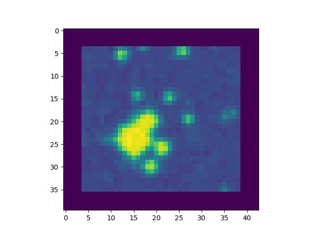
This must be added to the file ex3_peaks.py.
Signature
The characteristics (width, height, sum) of the extended image
signature_fmt_3 = 'RESULT: extended_image_width = {:d}'
signature_fmt_4 = 'RESULT: extended_image_height = {:d}'
signature_fmt_5 = 'RESULT: extended_image_sum = {:.0f}'
If you want to check your program with the common image common.fits, here is
the expected signature:
RESULT: extended_image_width = 282
RESULT: extended_image_height = 160
RESULT: extended_image_sum = 198911082
Step 3: build the convoluted image#
In this step, you will implement an image scan to build the convoluted image. This image scan is done pixel by pixel, row by row (first row, then second row…).
The scan main characteristics are:
For each pixel, the 9x9 gaussian pattern (convolution matrix) has to be applied to a 9x9 sub-image centered at the scanned location. To be able to apply the pattern on the borders, you have extended the image to add a margin whose size is half the pattern width (4 in our case). This way, all pixels in the original image do have neighbours in all directions. However, you should be careful to only perform the scan over the pixels of the original image.

To extract a sub-image from the image, when this image is stored in a
Numpyarray, you need to use the following slicing expression:sub_image = image[top-row:bottom-row, left-column:right-column]
As for slices in Python, the first value of each dimension (
top-row,left-column) is the first index that will be part of the sub-image. The second one (bottom-row,right-column) is the first index to be excluded.To compute the scalar value of the convolution at each position, the gaussian pattern (kernel) is convoluted with the sub-image centered at this position, then all the pixel values of the convoluted sub-image are summed up.
This is typically done with the
numpy.sum()function that returns the sum of all the matrix elements:convolution = np.sum(sub_image * pattern)
When the scan position is close to the extended margin, the pattern will be partly applied to the image pixels and partly to the margin pixels, introducing some error in the cluster characteristics, in particular its luminosity. This error will be considered negligible in our context.
Signature
The characteristics (width, height, sum) of the convoluted image
signature_fmt_6 = 'RESULT: convoluted_image_width = {:d}'
signature_fmt_7 = 'RESULT: convoluted_image_height = {:d}'
signature_fmt_8 = 'RESULT: convoluted_image_sum = {:.0f}'
If you want to check your program with the common image common.fits, here is
the expected signature:
RESULT: convoluted_image_width = 274
RESULT: convoluted_image_height = 152
RESULT: convoluted_image_sum = 196347878
Warning
The original image is a numpy array made of int values. On the contrary, the
convolution pattern should be a numpy array made of float values, and so the
convoluted image. If you store your convoluted image as a numpy array made of
int, your convoluted_image_sum in the signature above will be wrong.
Display#
In the application display.py, you may want to display the convoluted image
side by side with the original one and check the visual effect of the
convolution: it should be blurred (less noise).
Step 4: extend the convolution image#
Back to ex3_peaks.py
Similarly to what had been done to extend the image, the peak finding algorithm will need accessing one single row of pixels around all visited pixels. Therefore we extend the convolution image by one one pixel wide margin all around it.
Signature
The characteristics (width, height, sum) of the extended convoluted image
signature_fmt_9 = 'RESULT: extended_convoluted_image_width = {:d}'
signature_fmt_10 = 'RESULT: extended_convoluted_image_height = {:d}'
signature_fmt_11 = 'RESULT: extended_convoluted_image_sum = {:.0f}'
If you want to check your program with the common image common.fits, here is
the expected signature:
RESULT: extended_convoluted_image_width = 276
RESULT: extended_convoluted_image_height = 154
RESULT: extended_convoluted_image_sum = 196347878
Step 5: identify the peaks#
You will finally identify the pixels that are peaks. A pixel is a peak if its value is strictly greater than the value of all its direct neighbours (i.e. the 8 pixels around it).
To achieve this you will need to scan the convoluted image, in the same way as in the previous step
(pixel by pixel, one row after the other) and write a function is_peak() which, for each pixel, will
return if it is a peak or not (considering only peaks above the threshold).
We only consider peak that are strictly above a threshold. The threshold takes into account the background evaluation done in previous exercise (together with the dispersion). You will use this following threshold expression so as to clearly exclude the background :
threshold = background + 6.0 * dispersion
Warning
Do reuse the background and dispersion made from the orginal raw image, as done in the previosu exercise. DO NOT compute new values from the concoluted images.
The image below illustrates the peak locations found for an image with 1 cluster:
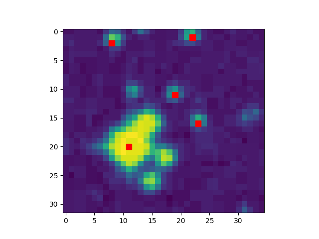
For your image you will construct a list of all peaks.
For a first validation of the peaks you found, you can visually check in the displayed image if they roughly match the “spots” you see.
Signature
First, the number of peaks found in the image,
signature_fmt_12 = 'RESULT: peaks_number = {:d}'
Then, the value, column and row of the peak with greatest value (in the convoluted image) :
signature_fmt_13 = 'RESULT: peak_max_value = {:.0f}'
signature_fmt_14 = 'RESULT: peak_max_column = {:d}'
signature_fmt_15 = 'RESULT: peak_max_row = {:d}'
If you want to check your program with the common image common.fits, here is
the expected signature:
RESULT: peaks_number = 118
RESULT: peak_max_value = 18508
RESULT: peak_max_column = 171
RESULT: peak_max_row = 111
Display#
In the application display.py, try to put a red dot or cross on the peaks
of the convoluted image, and/or the original image.
